Getting Started with PyMicrostructure
PyMicrostructure is designed with a modular structure, allowing you to easily create and customize market simulations. The main components of the library interact as follows:
Markets: The core of the simulation. They manage the order book, execute trades, and maintain the state of the market.
Traders: Entities that interact with the market by submitting orders.
Orders: Instructions to buy or sell assets, submitted by traders to the market.
Strategies: Customizable strategies that determine how traders make decisions.
Metrics: Tools to analyze the performance of the market and individual traders.
Visualization: Functions to create visual representations of the simulation results.
Basic Simulation Example
Let’s walk through a simple example to demonstrate how these components work together:
from pymicrostructure.markets.continuous import ContinuousDoubleAuction
from pymicrostructure.traders.market_maker import DummyMarketMaker
from pymicrostructure.traders.noise import NoiseTrader
from pymicrostructure.visualization.summary import participant_comparison, price_path

# 1. Create a market
market = ContinuousDoubleAuction(initial_fair_price=1000)

# 2. Create traders
mm = DummyMarketMaker(market)
nt = NoiseTrader(market)

# 3. Run the simulation
market.run(500)

# 4. Visualize the results
participant_comparison(market.participants)
price_path(market)
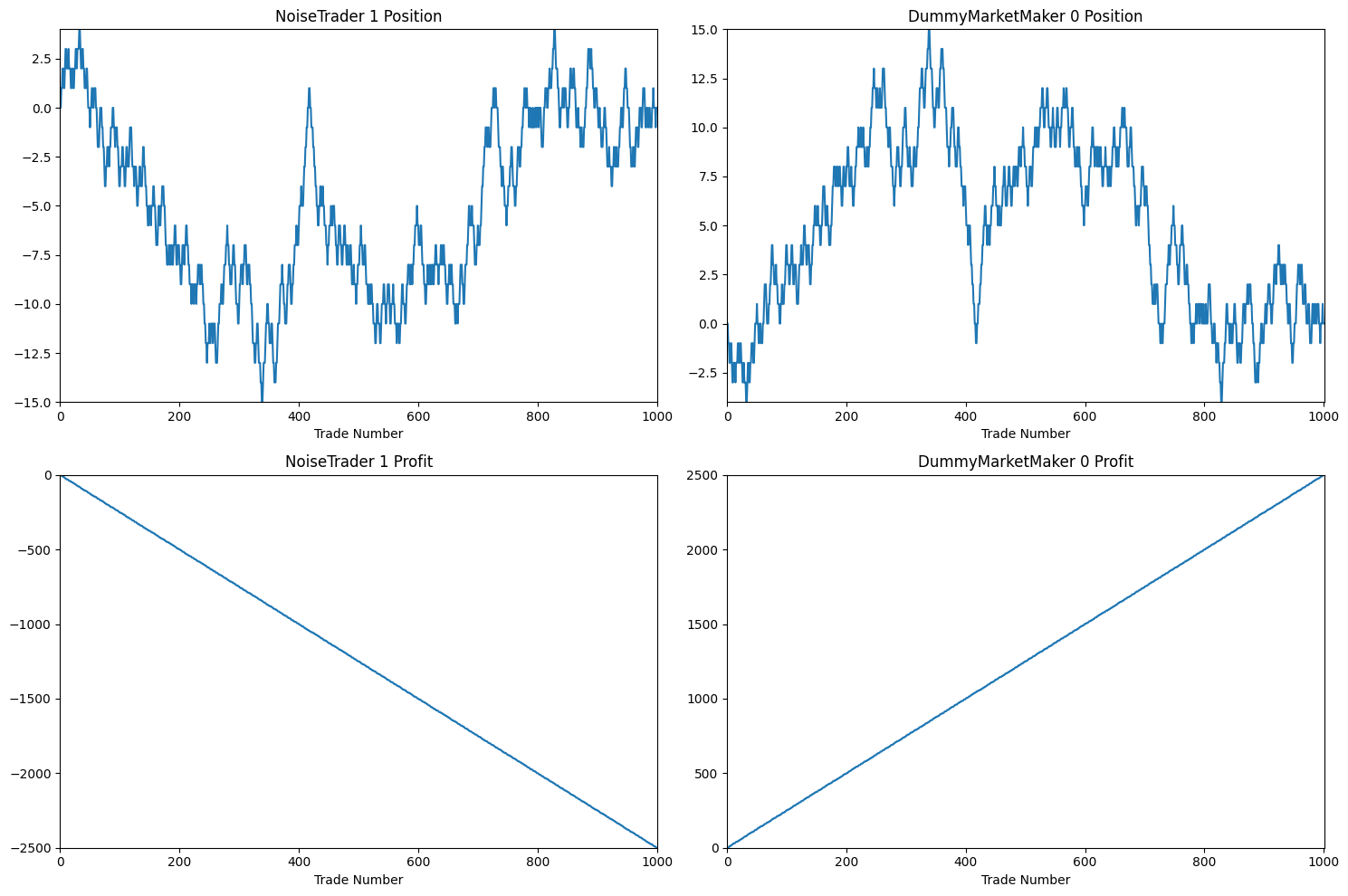
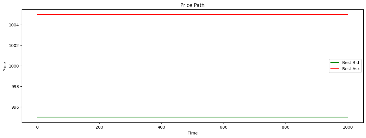
In this example, because DummyMarketMaker holds constant spread and fair price estimate, we see the bid and ask price not moving for the entirety of trading.
This, combined with the fact that he is the only market maker and NoiseTrader submits random market orders, causes the market maker to make consistent profit.
We can view details of the final performances of the traders with participants_report:
from pymicrostructure.metrics.trader import participants_report

participants_report(market.participants)
NoiseTrader_1 |
DummyMarketMaker_0 |
|
|---|---|---|
final_profit |
-2500 |
2500 |
final_position |
0 |
0 |
profit_per_state |
-2.5 |
2.5 |
std_profit_per_state |
2.5 |
2.5 |
information_ratio |
-1 |
1 |
total_trades |
500 |
500 |
volume_traded |
500 |
500 |
profit_per_volume |
-5 |
5 |
average_trade_size |
1 |
1 |
fill_rate |
1 |
0 |
time_in_market |
0.91 |
0.91 |
mean_position |
-4.97 |
4.97 |
mean_abs_position |
5.38 |
5.38 |
volume_as_aggressor |
500 |
0 |
volume_as_passive |
0 |
500 |
aggressor_ratio |
1 |
0 |
Congratulations! You just simulated and analyzed your first trading session with PyMicrostructure!
Using Trader Templates: Creating a Kyle-like Market
PyMicrostructure has multiple pre-built trader templates to choose from. This example goes through a simple Kyle-like market. We’ll set up a continuous double auction market with three types of traders: a Kyle-style market maker, an informed trader, and a noise trader.
First, import the necessary modules:
from pymicrostructure.markets.continuous import ContinuousDoubleAuction
from pymicrostructure.traders.market_maker import *
from pymicrostructure.traders.informed import *
from pymicrostructure.traders.noise import *
from pymicrostructure.visualization.summary import participant_comparison, price_path
from pymicrostructure.metrics.trader import participants_report
Initialize the market:
market = ContinuousDoubleAuction(initial_fair_price=1000)
Create the traders:
mm = KyleMarketMaker(market)
informed = TWAPInformedTrader(market)
noise = NoiseTrader(market, submission_rate=1, volume_size=lambda: np.random.randint(5, 20))
Note that submission_rate for noise trader indicates how often will noise trader submit a trade,
and volume_size indicates sizes of orders they submit (can be a constant or lambda to make it random).
Run the market simulation for 300 time steps:
market.run(300)
Generate visualizations to analyze the results:
participant_comparison(market.participants)
price_path(market)
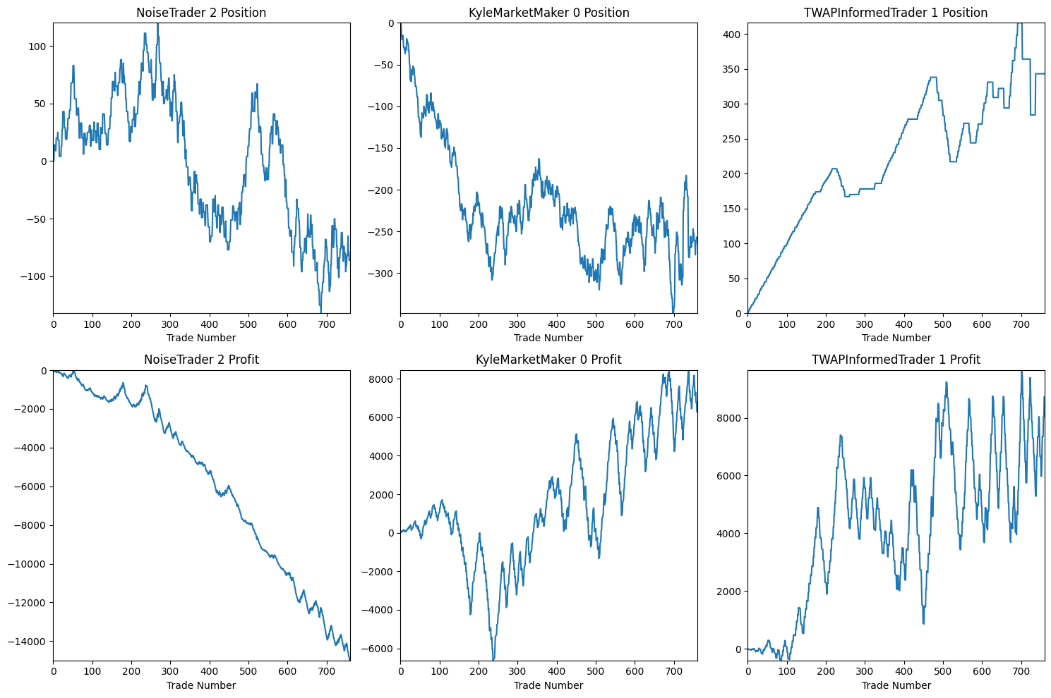
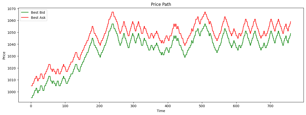
A comparison of profits and losses for each trader. The price path, starting at 1000 and stabilizing at 1050 (the informed trader’s target price).
Generate a report of trader metrics:
participants_report(market.participants)
NoiseTrader_2 |
KyleMarketMaker_0 |
TWAPInformedTrader_1 |
|
|---|---|---|---|
final_profit |
-15000 |
6281 |
8719 |
final_position |
-86 |
-257 |
343 |
profit_per_state |
-19.76 |
8.28 |
11.49 |
std_profit_per_state |
80.07 |
296.99 |
309.95 |
information_ratio |
-0.25 |
0.03 |
0.04 |
total_trades |
300 |
459 |
159 |
volume_traded |
3556 |
4641 |
1085 |
profit_per_volume |
-4.22 |
1.35 |
8.04 |
average_trade_size |
11.85 |
10.11 |
6.82 |
fill_rate |
1 |
0.08 |
1 |
time_in_market |
1 |
1 |
1 |
mean_position |
-1.53 |
-218.72 |
220.25 |
mean_abs_position |
49.04 |
218.72 |
220.25 |
volume_as_aggressor |
3556 |
0 |
1085 |
volume_as_passive |
0 |
4641 |
0 |
aggressor_ratio |
1 |
0 |
1 |
In this example:
The Kyle-style market maker (KyleMarketMaker_0) achieves a positive profit after initial setback, demonstrating its ability to learn from order flow.
The informed trader (TWAPInformedTrader_1) also profits, as expected given its information advantage.
The noise trader (NoiseTrader_2) loses money, which is typical for random trading strategies. The price path stabilizing at the informed trader’s target price (1050) shows how information is gradually incorporated into the market price through the interactions of these different trader types. This simple example demonstrates how PyMicrostructure’s trader templates can be used to create and analyze complex market dynamics with just a few lines of code.
Building New Traders with Strategies Module
We can now try to create a more custom Trader with strategy module. We’ll set up a market with a custom market maker, an informed trader, and a noise trader, and then analyze their performance.
Apart from previous imports, let’s add:
from pymicrostructure.traders.strategy import *
Now, we’ll create our market, pre-defined traders and custom market-maker:
market = ContinuousDoubleAuction(initial_fair_price=1000)

mm = BaseMarketMaker(market,
                     fair_price_strategy=OrderFlowMagnitudeFairPrice(window=10, aggressiveness=1),
                     volume_strategy=MaxFractionVolume(fraction=0.1),
                     spread_strategy=OrderFlowImbalanceSpread(window=5, aggressiveness=10, min_halfspread=3),
                     max_inventory=1000)

informed = TWAPInformedTrader(market)
noise = NoiseTrader(market, submission_rate=1, volume_size=lambda:np.random.randint(1, 5))
Let’s break down what’s happening here:
We create a BaseMarketMaker to which we pass three new things:
fair_price_strategy=OrderFlowMagnitudeFairPrice(window=10, aggressiveness=1)sets the fair price based on the order flow magnitude over a 10-tick window with an aggressiveness of parameter of 1.volume_strategy=MaxFractionVolume(fraction=0.1)sets the maximum volume to 10% of the trader’s maximum possible volume.spread_strategy=OrderFlowImbalanceSpread(window=5, aggressiveness=10, min_halfspread=3)sets the spread based on the order flow imbalance over a 5-tick window with an aggressiveness of 10 and a minimum half-spread of 3.
Now we can run our market simulation:
market.run(300)
After the simulation, we can visualize and analyze the results:
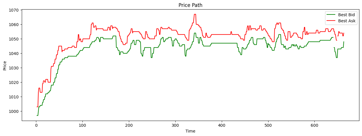
participant_comparison(market.participants)
price_path(market)
participants_report(market.participants)
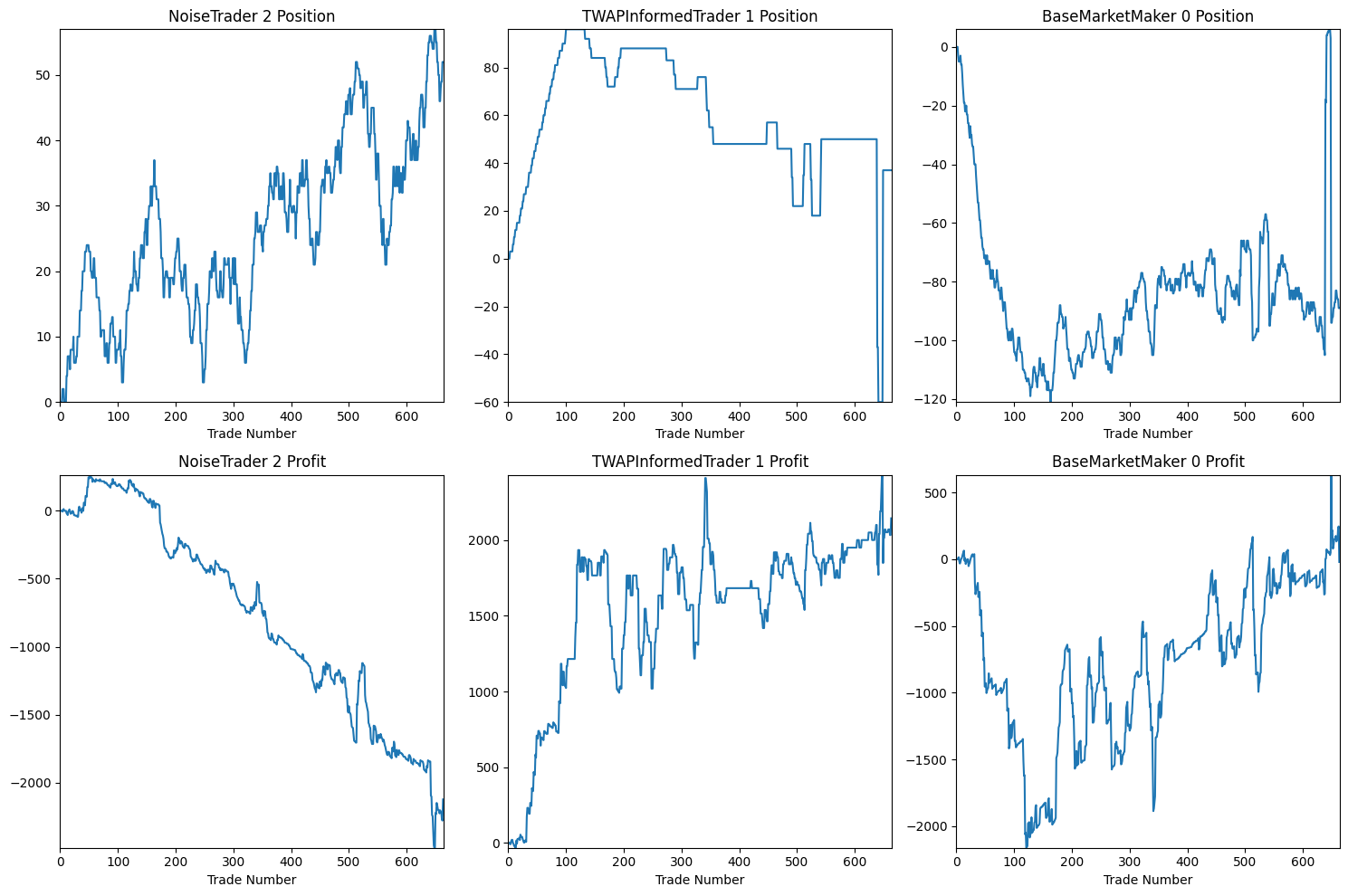
NoiseTrader_2 |
TWAPInformedTrader_1 |
BaseMarketMaker_0 |
|
|---|---|---|---|
final_profit |
-2124 |
2145 |
-21 |
final_position |
52 |
37 |
-89 |
profit_per_state |
-3.2 |
3.24 |
-0.03 |
std_profit_per_state |
32.78 |
68.18 |
89.65 |
information_ratio |
-0.1 |
0.05 |
-0 |
total_trades |
299 |
63 |
362 |
volume_traded |
758 |
525 |
1283 |
profit_per_volume |
-2.8 |
4.09 |
-0.02 |
average_trade_size |
2.54 |
8.33 |
3.54 |
fill_rate |
1 |
0.84 |
0.02 |
time_in_market |
0.99 |
1 |
1 |
mean_position |
26.15 |
58.26 |
-84.41 |
mean_abs_position |
26.15 |
59.93 |
84.53 |
volume_as_aggressor |
758 |
525 |
0 |
volume_as_passive |
0 |
0 |
1283 |
aggressor_ratio |
1 |
1 |
0 |
We can also analyze specific market metrics, such as the quoted spread:
from pymicrostructure.metrics.market import quoted_spread

quoted_spread(market).plot()
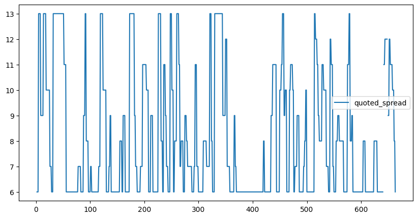
This will plot the quoted spread over time, giving us insight into market liquidity dynamics.
This example demonstrates how PyMicrostructure can be used to create complex market simulations with different types of traders and custom strategies. By adjusting the parameters and strategies, you can explore a wide range of market scenarios and trader behaviors.
Key points to note:
The market maker adapts its fair price, volume, and spread based on market conditions.
The informed trader uses a TWAP strategy to execute its trades.
The noise trader adds randomness to the market, simulating uninformed participants.